


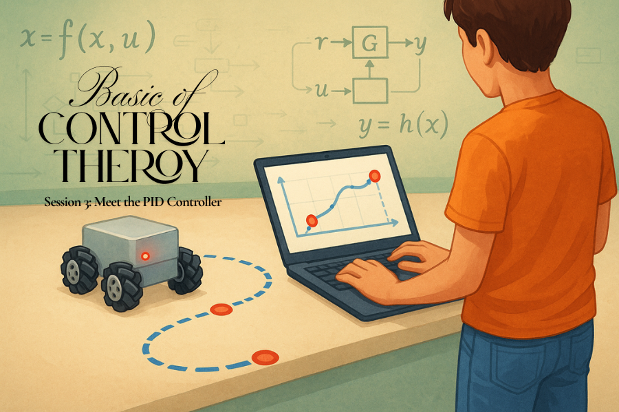
Welcome back to our journey into the world of control theory! So far, we’ve established that we are all natural-born control systems experts, and we’ve unpacked the crucial difference between a “trusting” open-loop system and a “verifying” closed-loop system. For our mecanum robot project—and for any task that demands precision and adaptability—we know that a closed-loop system is the only way to go.
This brings us back to our four magic words: Measure, Compare, Compute, Correct. We know we need to measure the state of our system (like the speed of a wheel) and compare it to our goal. But what happens next? How does the controller compute the right correction?
This is where the real intelligence of the system lies. It’s not magic; it’s an elegant and powerful algorithm that acts as the system’s brain. Today, we’re going to meet the undisputed champion of the control world, the algorithm used in everything from thermostats to self-driving cars: the Proportional-Integral-Derivative (PID) controller.
The Fuel of Control: The Error Signal
Before we meet the PID team, let’s give a name to the thing that drives them. In Session 2, we talked about the “difference” between the desired value and the actual value. In control theory, this is called the error. We can define it with a simple, powerful equation:
\(e(t) = r(t) - y(t)\)Here, e(t) is the error at a given time t. The term r(t) is the reference or setpoint (what you want), and y(t) is the measured output of the system (what you’ve got). This error signal, e(t), is the single piece of information that the PID controller uses to make all of its decisions.
The entire goal of the controller is to compute a correction that will drive this error to zero over time. It does this using a combination of three different strategies, all rolled into one equation. The full PID formula looks like this:
\(u(t) = K_p \, e(t) + K_i \int_{0}^{t} e(\tau) \, d\tau + K_d \frac{d}{dt}e(t)\)Don’t let the symbols intimidate you! This is just a formal way of saying that the correction, u(t), is the sum of three parts. Let’s break it down by thinking of it not as one complex brain, but as a team of three specialists, each with a unique personality and job.
P is for Proportional: The “Right Now” Specialist
The Proportional controller is the most straightforward of the three. Its philosophy is simple: the bigger the error, the bigger the correction. Its contribution is calculated as:
\(P_{\text{out}} = K_p \, e(t)\)Here, KP is the “proportional gain,” a tuning knob that dictates how aggressively it reacts. Imagine you are pushing a friend on a playground swing. If the swing is very far from its target height (a large error), you give it a big push. If it’s close (a small error), you only need a gentle nudge. The P-controller does exactly this, providing the primary muscle to get the system moving toward its goal.
The Downside: The P-controller has a critical weakness. As the system gets closer to the target, the error gets smaller, and so its push gets weaker. Eventually, the push is too weak to overcome forces like friction, resulting in a small but permanent steady-state error. It gets the system almost there, but not quite.
I is for Integral: The Grudge-Holding Historian
This is where the Integral specialist steps in. The I-controller isn’t concerned with the present moment; it’s obsessed with the past. It looks at the accumulated error over time. Its part of the equation is:
\(I_{\text{out}} = K_i \int_{0}^{t} e(\tau) \, d\tau\)Think of the I-controller as someone with a long memory. That small, steady-state error left by the P-controller? The I-controller sees it. The longer that error persists, the more “frustrated” the I-controller gets. It sums up the error over time (the integral), and this sum grows and grows. Eventually, this accumulated value gets so large that the I-controller adds a powerful corrective action to finally wipe out that lingering error for good.
The Downside: The I-controller’s focus on the past can make it overshoot the target. Because it has built up all this corrective momentum, it might still be pushing hard even after the error has reached zero, causing the system to swing past the setpoint. This is a phenomenon known as “integral windup”.
D is for Derivative: The Future-Predicting Strategist
So, how do we create a smooth, stable response? We bring in our third specialist: the Derivative controller. The D-controller is the forward-thinker. It only cares about one thing: how fast the error is changing. It calculates the rate of change (the derivative) of the error to predict where the error will be in the near future.
\(D_{\text{out}} = K_d \frac{d}{dt} e(t)\)Its job is to act as a damper. If it sees the error is closing very quickly, it predicts an overshoot is coming. In response, it applies a counteracting force, like tapping the brakes as you approach a stoplight. This “anticipation” slows the system down as it nears the target, significantly reducing overshoot and smoothing out oscillations.
The Downside: The D-controller is extremely sensitive to noise. A jumpy sensor can cause tiny, rapid changes in the error, which the D-controller interprets as massive rates of change. This can cause it to overreact, making the system unstable.
The Perfect Team: Tuning the PID
The magic of a PID controller is how these three specialists work together. The final output is the sum of their individual efforts.
- P provides the main response based on the current error.
- I looks back in time to eliminate any final, steady-state error.
- D looks to the future to dampen the response and prevent overshoot.
The process of getting this team to work in harmony is called tuning. Tuning involves adjusting the gains for each component—KP , Ki , Kd —which determines how much influence each specialist has on the final decision. Finding the right balance is the key to creating a control system that is fast, accurate, and stable.
Back to Our Robot
Let’s apply this to one of our mecanum robot’s wheels. Our goal is to make it spin at exactly 100 RPM.
- We send a command. The wheel starts spinning, but our encoder (Measure) reports it’s only at 70 RPM. The controller (Compare) calculates an error of 30 RPM.
- The P-controller sees this big error and immediately commands a large increase in motor power. The speed jumps to 98 RPM. The error is now only 2 RPM, so the P-controller’s push becomes much weaker.
- The wheel is now stuck at a steady 98 RPM. The I-controller, seeing this persistent 2 RPM error, starts accumulating it. After a moment, its “frustration” builds, and it adds extra power to the motor, pushing the speed up toward 100 RPM.
- As the speed rapidly accelerates from 98 to 100 RPM, the D-controller sees the error is closing fast. It predicts an overshoot and applies a small braking force, easing off the power just enough so the wheel settles smoothly at 100 RPM instead of flying past it to 105 RPM.
The result? A wheel that gets to its target speed quickly, accurately, and without wild oscillations. Now, imagine this happening for all four wheels at once, hundreds of times a second. That is the power of PID control.
What’s Next?
We now have the “brain” of our controller figured out. We understand the theory of how to compute a correction. But before we can apply this brain, we need to understand the body. In our next session, we’ll dive into the physics of our robot. We’ll explore the fascinating world of kinematics—the geometry of motion—to understand how the individual speeds of our four special mecanum wheels translate into movement in any direction. Get ready to turn theory into physical motion!


